3D Cantilever Beam Simulation

We can make a 3D cantilever beam simulation almost identically to how we made the 2D cantilever beam. We start by defining a mesh for a beam:

from __future__ import print_function
import numpy as np
import region_selector_3d as rs
from dolfin import *

length = 20.0 # [mm]
width = 2.0 # [mm]
thickness = 1.0 # [mm]
resolution = 2 # [Nodes/mm]

resX = int(resolution * length) # Num nodes in x axis
resY = int(resolution * width) # Num nodes in y axis
resZ = int(resolution * thickness) # Num nodes in z axis

mesh = BoxMesh(Point(0.0,0.0,0.0), Point(length, width, thickness), resX, resY, resZ)

We will now label the fixed and load regions using region_selector_3d. We will fix the face at \(x=0\) and apply the load on the last 1mm on the top face of the beam furthest from the fixed end:

fixedRegion = rs.GetPlanarBoundary.from_coord('x', 0.0)
loadRegion = rs.GetPlanarBoundary.from_points(\
    Point(length, 0.0, thickness),\
    Point(length, width, thickness),\
    Point(length - 1.0, width, thickness),\
    Point(length - 1.0, 0.0, thickness))

boundaries = MeshFunction('size_t', mesh, mesh.topology().dim()-1)
boundaries.set_all(0)
fixedRegion.mark(boundaries,1)
loadRegion.mark(boundaries,2)

folder_name = './3d_cantilever_results'
boundaryfile = File('%s/boundaries.pvd' % folder_name
boundaryfile << boundaries

ds = Measure('ds', domain = mesh, subdomain_data = boundaries)

ParaView lets us see our defined domains.

We can see that the entire near face is marked 1, and the final milimeter of the top face is labeled 2, matching our description. The rest of the code is nearly identical to the 2D cantilever beam simulation. In this example we’ll be showing how to adjust the load to more closely represent a single load, in this case \(-5 \text{N}\) in the Z direction, rather than the load distribution that was used in the 2D example. We will define our desired load in \(\text{N}\) and then convert it to \(\frac{\text{N}}{\text{mm}^2}\) by dividing by the area of the load region. This only works when the mesh marked load region and the region selector class match exactly.

E = 68900.0 # [N/mm^2]
nu = 0.33 # Poisson's ratio
mu = E / (2.0 * (1.0 + nu))
lmbda = E*nu / ((1.0 + nu) * (1.0-2.0*nu))

load = Constant((0.0,0.0,-5.0)) # [N]
loadArea = loadRegion.area()
scaledLoad = load / loadArea

def eps(u):
    return sym(grad(u))

def sigma(u):
    return lmbda*tr(eps(u)) * Identity(mesh.topology.dim()) + 2.0*mu*eps(u)

V = VectorFunctionSpace(mesh, "Lagrange", 1)
du = TrialFunction(V)
u = Function(V, name="Displacement")
v = TestFunction(V)

a = inner(sigma(du), eps(v))*dx
L = dot(scaledLoad,v)*ds(2)

bc = DirichletBC(V, Constant((0.0,0.0,0.0)), fixedRegion)

solve(a == L, u, bc)

u.rename("Displacement", "Displacement")
xdmf_file = XDMFFile('%s/results.xdmf' % folder_name)
xdmf_file.write(u,1.0)

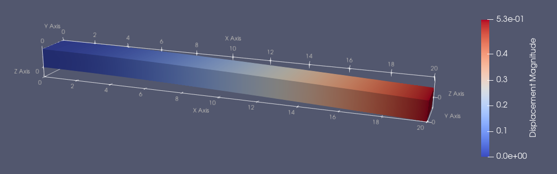
Our simulation indicates that under a \(5 \text{N}\) downwards load, a cantilevered aluminum beam (E = \(68900 \frac{\text{N}}{\text{mm}^2}\), nu = \(0.33\)) that is \(20\text{mm}\) long, \(2\text{mm}\) wide, and \(1\text{mm}\) thick will deflect about \(0.53\text{mm}\) downwards. Let’s compare that to Autodesk Inventor’s stress analysis simulation:

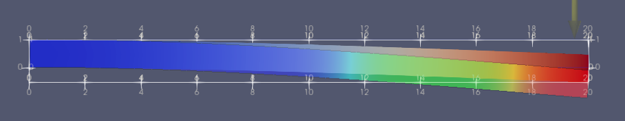
The rainbow colored one is from Inventor. So why do the results disagree so much? It seems like the Inventor simulation has the beam displace about twice as much. The reason is that specified a linear shape function to interpolate the solution between the mesh nodes.

V = VectorFunctionSpace(mesh, "Lagrange", 1)

If we want a better approximation, we increase the number nodes per element by specifying the order of the interpolating polinomial function. If we change the shape function from a linear to a quadratic approximation, we write

V = VectorFunctionSpace(mesh, "Lagrange", 2)

This makes the simulation more computationally expensive, since we have more nodes, but provide better results.

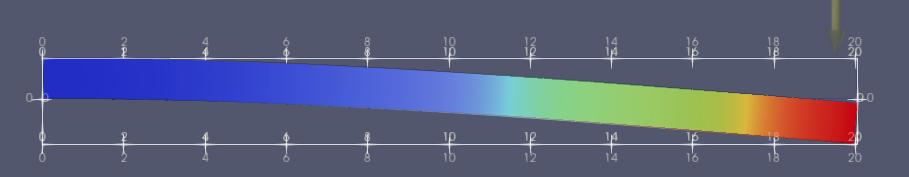
The new displacement, \(1.1\text{mm}\), matches the Euler-Bernoulli calculation for the deflection of this beam.

Complete Code

The complete code follows and can also be downloaded here.

from __future__ import print_function
import region_selector_3d as rs
from dolfin import *

length = 20.0 # [mm]
width = 2.0 # [mm]
thickness = 1.0 # [mm]
resolution = 2 # [Nodes/mm]

resX = int(resolution * length) # Num nodes in x axis
resY = int(resolution * width) # Num nodes in y axis
resZ = int(resolution * thickness) # Num nodes in z axis

mesh = BoxMesh(Point(0.0,0.0,0.0), Point(length, width, thickness), resX, resY, resZ)

fixedRegion = rs.GetPlanarBoundary.from_coord('x', 0.0)
loadRegion = rs.GetPlanarBoundary.from_points(\
    Point(length, 0.0, thickness),\
    Point(length, width, thickness),\
    Point(length - 1.0, width, thickness),\
    Point(length - 1.0, 0.0, thickness))

boundaries = MeshFunction('size_t', mesh, mesh.topology().dim()-1)
boundaries.set_all(0)
fixedRegion.mark(boundaries, 1)
loadRegion.mark(boundaries, 2)

ds = Measure('ds', domain=mesh, subdomain_data=boundaries)

folder_name = './3d_cantilever_results'
    
boundaryfile = File('%s/boundaries.pvd' % folder_name)
boundaryfile << boundaries

E = 68900.0 # [N/mm^2]
nu = 0.33 # Poisson's ratio
mu = E / (2.0 * (1.0 + nu))
lmbda = E*nu / ((1.0 + nu) * (1.0-2.0*nu))

load = Constant((0.0,0.0,-5.0)) # [N]
# Convert to N/mm
loadArea = loadRegion.area()
scaledLoad = load / loadArea

def eps(u):
    return sym(grad(u))

def sigma(u):
    return lmbda*tr(eps(u)) * Identity(mesh.topology().dim()) + 2.0*mu*eps(u)

V = VectorFunctionSpace(mesh, "Lagrange", 1)
du = TrialFunction(V)
u = Function(V, name="Displacement")
v = TestFunction(V)

a = inner(sigma(du), eps(v))*dx
L = dot(scaledLoad,v)*ds(2)

bc = DirichletBC(V, Constant((0.0,0.0,0.0)), fixedRegion)

solve(a == L, u, bc)

u.rename("Displacement", "Displacement")
xdmf_file = XDMFFile('%s/results.xdmf' % folder_name)
xdmf_file.write(u,1.0)