2D Cantilever Optimization
Introduction
Suppose we want to make an aluminum shelf no taller than 10cm to best support an \(4\text{cm}\) wide and \(80\text{cm}\) long rod weighing \(500\text{N}\) \(23\text{cm}\) away from a wall while keeping the mass of the shelf under \(16.2\text{kg}\). This shelf will simply be a 2D profile extruded out of the page \(80\text{cm}\) for ease of manufacturing, so we can just focus on optimizing the 2D profile. In order to ensure the rod is supported, we require that \(1\text{cm}\) of material is present under it through its whole width. What is the best shape for the shelf to have? The design space can be summarized in a sketch:
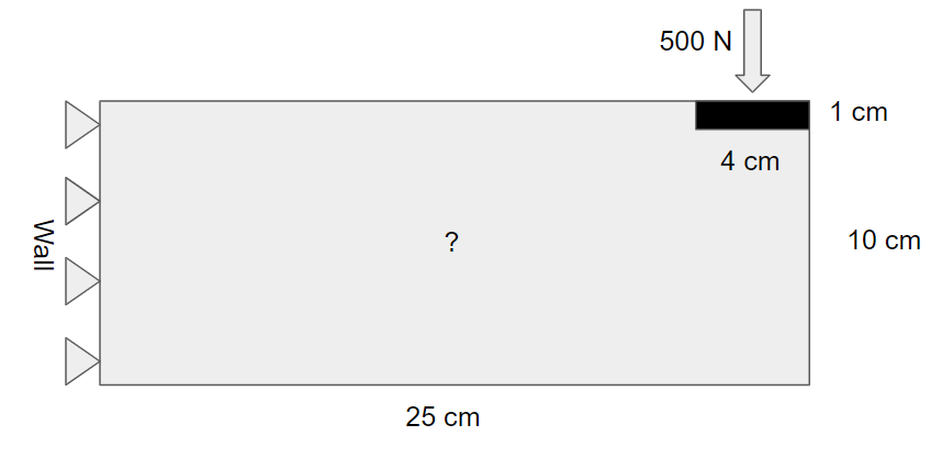
This is known as the design domain of the problem. We want to figure out how to best support the rod while keeping the total mass of the shelf under \(16.2\text{kg}\). How do we express this mathematically? First, let’s find what fraction of our design domain can be filled with material. At any location, we can either have aluminum or not - there is no partial density. This means that \(16.2\text{kg} * \frac{1 \text{cm}^3}{2.7 g} = 6000 \text{cm}^3\) can be filled with aluminum, which works out to \(\frac{6000 \text{cm}^3}{25\text{cm} * 10\text{cm} * 80 \text{cm}} = .3\), so up to 30% of the design domain can be filled with aluminum. We also need to define “best support” as an objective function. We can do this by minimizing the compliance which can be defined as the sum of the strain energy in the part. Since we are operating in the elastic region we know that the strain energy in the part is equal to the input energy, or
Where \(\boldsymbol{F}\) represents the applied forces at the subsurfaces \(\text{dA}\) on the applied load region \(\Omega\) and \(\boldsymbol{v}\) represent the displacements on \(\text{dA}\). Importantly, \(\text{J}\) is a single scalar value so it is simple to optimize. \(\text{J}\) is a function of \(\boldsymbol{\rho}\), the density distribution in the region, which is a continuous value between 0 and 1. In the end we ideally want \(\boldsymbol{\rho}\) to converge to 0 or 1 on each element. In summary, we want to vary \(\boldsymbol{\rho} \in [0,1]\) to minimize \(\text{J}(\boldsymbol{\rho})\) while keeping \(\int_V \rho \text{dV} < 0.3\int_V 1 \text{dV}\), where V is the domain space. Further, \(\forall (x,y | x \in [21, 25] \cap y \in [9, 10]) \rightarrow \boldsymbol{\rho}(x,y) = 1\). In order to avoid the checkerboard problem we will add a filter term to \(\text{J}\) to penalize too many changes in \(\boldsymbol{\rho}\) with a weight, in this case
Implementation
We start by first defining a standard Dolfin model to find the displacements in a 2D profile when a load is applied, much like the 2D Cantilever example, but this time this displacement will be as a function of a scalar function \(\boldsymbol{\rho}\). We will use a load of \(500\text{N}\), though the specific value of the load should not matter too much on the final result of the optimization as long as it isn’t far too small or far too great. We start by defining the material properties, loads, mesh, and regions:
from __future__ import print_function
import numpy as np
import region_selector_2d as rs
from dolfin import *
from dolfin_adjoint import *

E = 69000.0 # N/mm^2
nu = 0.33
mu = E / (2.0*(1.0 + nu))
lmbda = E*nu / ((1.0 + nu) * (1.0 - 2.0*nu))

folder_name = './2d_cantilever_opt_results'

length = 250.0 # [mm]
thickness = 100.0 # [mm]
resolution = .2 # [Nodes/mm]
load = Constant((0.0,-500.0)) # [N]

resX = int(resolution * length) # Num nodes in x axis
resY = int(resolution * thickness) # Num nodes in y axis

mesh = RectangleMesh(Point(0.0,0.0), Point(length, thickness), resX, resY, 'crossed')

fixedRegion = rs.GetLinearBoundary.from_points(Point(0.0,0.0), Point(0.0,thickness))
loadRegion = rs.GetLinearBoundary.from_points(Point(length-40.0, thickness), Point(length, thickness))

boundaries = MeshFunction('size_t', mesh, mesh.topology().dim() - 1)
boundaries.set_all(0)
fixedRegion.mark(boundaries, 1)
loadRegion.mark(boundaries, 2)

boundaryfile = File('%s/simpleBoundaries.pvd' % folder_name)
boundaryfile << boundaries
We will now define a region for the “frozen” region where the load is applied and \(\boldsymbol{\rho} = 1\):
domains = MeshFunction('size_t', mesh, mesh.topology.dim())
frozenLoadRegion = rs.GetRectangularRegion.from_points(Point(length, thickness), Point(length - 40.0, thickness - 10.0))

domains.set_all(0)
frozenLoadRegion.mark(domains, 1)

domainfile = File('%s/simpleDomains.pvd' % folder_name)
domainfile << domains

ds = Measure('ds', domain=mesh, subdomain_data=boundaries)
dx = Measure('dx', domain=mesh, subdomamin_data=domains)

loadArea = assemble(Constant(1.0)*ds(2))
scaledLoad = load / loadArea

# Function space for displacements
V = VectorFunctionSpace(mesh, "Lagrange", 1)
# Function space for rho
V0 = FunctionSpace(mesh, "Lagrange", 1)
Now we create the forward_linear function, which takes in a value for the \(\boldsymbol{\rho}\) distribution in the region and the boundary conditions and returns the displacements. This requires an adaptation to the sigma method and an additional method to “encourage” the \(\boldsymbol{\rho}\) values to tend towards 0 or 1, with a limit on how close the values can get to 0 to avoid division errors. The forward_linear function uses the values on dx to separately evaluate the non-frozen regions which will use the passed in \(\boldsymbol{\rho}\) values and the frozen regions which will always use \(\boldsymbol{\rho} = 1\)
p = 4.0 # Penalization factor
gamma = Constant(1e-2) # Min value

def alpha(rho): # Penalization on intermediate values
    return gamma + (1-gamma) * rho**p

def eps(u):
    return sym(grad(u))

def sigma(u, rho):
    return alpha(rho)*(lmda*tr(eps(u))*Identity(mesh.topology().dim()) + 2.0*mu*eps(u))

def forward_linear(rho, bcs):
    du = TrialFunction(V)
    u = Function(V, name = "Displacement")
    v = TestFunction(V)

    a = inner(sigma(du, rho), eps(v)) * dx(0) + inner(sigma(du, Constant(1.0)), eps(v)) * dx(1)
    L = dot(scaledLoad, v) * ds(2)

    solve(a == L, u, bcs)
    return u
We now set up the optimization. We first define the boundary conditions and an initial guess for \(\boldsymbol{\rho}\) and calculate the displacements for this guess:
bc = DirichletBC(V, Constant((0.0,0.0)), fixedRegion)

vf = 0.3 # Max volume fraction

# Initial guess: uniform density with max volume fraction
rho = interpolate(Constant(vf), V0)

# Solve initial displacement for initial guess
u = forward_linear(rho, bc)
Here we define a function which will be called after every step of the optimization. In this case we simply want it to print the current values for \(\boldsymbol{\rho}\) so we can watch the progress of the optimization.
iteration = File("%s/iterations.pvd" % folder_name)

# Runs after every optimization iteration
def derivative_cb(j, dj, m):
    m.rename("Densities", "Densities")
    iterations << m
We will now define the objective function and control for the minimization problem. Dolfin_adjoint uses the ReducedFunctional class to compute derivatives of the objective function with respect to the control, and it is what is used for the optimization:
# Weights for each part of obj function
dispW = Constant(1.0)
filterW = Constant(5.0e-1)

# Minimize strain energy
Jdisp = assemble(dispW * dot(load,u)*ds(2))
# Minimize gradient of rho
Jfilter = assemble(filterW * inner(grad(rho), grad(rho)) * dx(0))

J = Jdisp + Jfilter

# Define control
m = Constrol(rho)
m_bounds = (0.0,1.0)

# Define reduced functional
Jhat = ReducedFunctional(J, m, derivative_cb_post = derivative_cb)
We will now set the volume constraint on \(\boldsymbol{\rho}\). This VolumeConstraint class will enforce the condition that the fraction of the volume (or the integral of \(\boldsymbol{\rho}\) through the region) is less than a passed in volfrac, in this case 0.3.
class VolumeConstraint(InequalityConstraint):
    def __init__(self, volfrac):
        self.volfrac = volfrac
        self.smass = assemble(TestFunction(V0)*Constant(1.0)*dx)
        self.smassNotFrozen = assemble(TestFunction(V0)*Constant(1.0)*dx(0))
        self.smassFrozen = assemble(TestFunction(V0)*Constant(1.0)*dx(1))
        self.rhovec = Function(V0)
        self.rhovecFrozen = interpolate(Constant(1.0),V0)

    def function(self, m):
        from pyadjoint.reduced_functional_numpy import set_local
        set_local(self.rhovec, m) # Set rhovec to the control, rho
        integralNotFrozen = self.smassNotFrozen.inner(self.volfrac - self.rhovec.vector())
        integralFrozen = self.smassFrozen.inner(self.volfrac - self.rhovecFrozen.vector())

        return integralNotFrozen + integralFrozen # Keep this >= 0

    def jacobian(self, m):
        return [-self.smass]

    def output_workspace(self):
        return [0.0]
We can now finally define the minimization problem, set some parameters, and solve for \(\boldsymbol{\rho}\).
problem = MinimizationProblem(Jhat, bounds = m_bounds, constraints = VolumeConstraint(vf))
parameters = {"max_iter": 500, 'linear_solver': 'ma97', 'tol': 1e-3, 'acceptable_tol': 1e-3, 'acceptable_iter': 10}

solver = IPOPTSolver(problem, parameters = parameters)
rho_opt = solver.solve()
As this code is running we can open ParaView and open the iterations.pvd file to view the progress of the optimization. Note that the frozen region’s \(\boldsymbol{\rho}\) value is not 1 - this is because the values of \(\boldsymbol{\rho}\) in that region are never even read and are always set to 1 in calculations. In post processing we set these values to 1, compute the displacements one last time, and write the results to a file. We can also compute other metrics for evaluating the design. In this case, we will also compute the von Mises stress.
# Post Processing
u = forward_linear(rho_opt, bc)
u.rename("Displacement", "Displacement")

v2d = vertex_to_dof_map(V0)
index_inside_pad = []

# Mark all frozen regions
for i,x in enumerate(mesh.coordinates()):
    if frozenLoadRegion.inside(x,True): index_inside_pad.append(i)

rho_opt.vector()[v2d[index_inside_pad]] = Constant(1.0)
rho.assign(rho_opt)
rho.rename("Densities", "Densities")

# von Mises Stress
stress = sigma(u,rho)
s = stress - (1./3)*tr(stress)*Identity(2)  # deviatoric stress
von_Mises = sqrt(3./2*inner(s,s))
Vvm = FunctionSpace(mesh,'P',1)
von_Mises = project(von_Mises,Vvm)
von_Mises.rename("von Mises","von Mises")

xdmf_file = XDMFFile('%s/results.xdmf' % folder_name)

xdmf_file.parameters["flush_output"] = True
xdmf_file.parameters["functions_share_mesh"] = True
xdmf_file.parameters["rewrite_function_mesh"] = False
xdmf_file.write(rho, 1.0)
xdmf_file.write(u, 1.0)
xdmf_file.write(von_Mises,1.0)
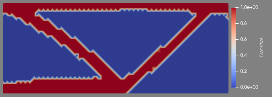
The post processed final shape is:
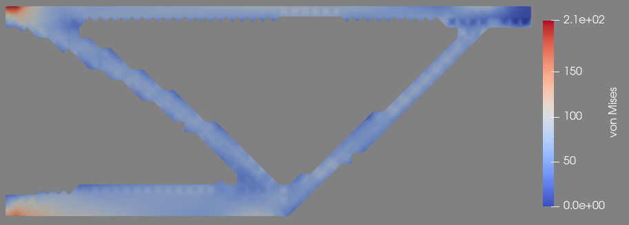
And when a threshold to only show the areas with \(\boldsymbol{\rho} > 0.8\) and change the coloring to von Mises Stress we get:
Complete Code
The complete code follows and can also be downloaded here.
# Example of using Fenics to model the bending of a simple cantilevered beam in 2D.

from __future__ import print_function
import numpy as np
import region_selector_2d as rs
from dolfin import *
from dolfin_adjoint import *

E = 69000.0 # N/mm^2 - aluminum 6061
nu = 0.3 # poisson's ratio
mu = E / (2.0*(1.0 + nu))
lmbda = E*nu / ((1.0 + nu) * (1.0 - 2.0*nu))

p = 4.0 # Penalization factor
gamma = Constant(1e-2) # Min value
vf = .3 # Fraction of volume allowed to be filled

length = 250.0 # [mm]
thickness = 100.0 # [mm]
resolution = .2 # [Nodes/mm] = 2 [Nodes/cm]
load = Constant((0.0,-500.0)) # [N]

folder_name = './2d_cantilever_opt_results'

resX = int(resolution * length) # Num nodes in x axis
resY = int(resolution * thickness) # Num nodes in y axis

# Boundary region for design
mesh = RectangleMesh(Point(0.0,0.0), Point(length, thickness), resX, resY, 'crossed')

# Function space for displacements
V = VectorFunctionSpace(mesh, "Lagrange", 1)
# Function space for rho
V0 = FunctionSpace(mesh, "Lagrange", 1)

# Load applied on the last 4cm on the top of the beam
loadRegion = rs.GetLinearBoundary.from_points(Point(length-40.0, thickness), Point(length, thickness))

# The end of the beam at x = 0 is fixed
fixedRegion = rs.GetLinearBoundary.from_points(Point(0.0,0.0), Point(0.0,thickness))

# Mark the fixed and node loads
boundaries = MeshFunction('size_t', mesh, mesh.topology().dim() - 1)
boundaries.set_all(0)
fixedRegion.mark(boundaries, 1)
loadRegion.mark(boundaries, 2)

boundaryfile = File('%s/simpleBoundaries.pvd' % folder_name)
boundaryfile << boundaries

domains = MeshFunction('size_t', mesh, mesh.topology().dim())
# The region within 1cm of the applied load is protected, rho forced to be 1
frozenLoadRegion = rs.GetRectangularRegion.from_points(Point(length, thickness), Point(length - 40.0, thickness - 10.0))

domains.set_all(0)
frozenLoadRegion.mark(domains, 1)

domainfile = File('%s/simpleDomains.pvd' % folder_name)
domainfile << domains

ds = Measure('ds', domain=mesh, subdomain_data=boundaries)
dx = Measure('dx', domain=mesh, subdomain_data=domains)

loadArea = assemble(Constant(1.0)*ds(2))
scaledLoad = load / loadArea

# Penalization on intermediate values
def alpha(rho):
    return gamma + (1-gamma)*rho**p

def eps(u):
    return sym(grad(u))

def sigma(u, rho):
    return alpha(rho)*(lmbda*tr(eps(u))*Identity(mesh.topology().dim()) + 2.0*mu*eps(u))

def forward_linear(rho, bcs):
    du = TrialFunction(V)
    u = Function(V, name="Displacement")
    v = TestFunction(V)

    a = inner(sigma(du, rho),eps(v))*dx(0) + inner(sigma(du, Constant(1.0)), eps(v))*dx(1)
    L = dot(scaledLoad,v)*ds(2)

    solve(a == L, u, bcs)
    return u

bc = DirichletBC(V, Constant((0.0,0.0)), fixedRegion)

# Initial guess: uniform density with max volume fraction
rho = interpolate(Constant(vf), V0)

# Solve initial displacement for the initial guess
u = forward_linear(rho, bc)

iterations = File("%s/iterations.pvd" % folder_name)

# Runs after every optimization iteration
def derivative_cb(j, dj, m):
    # Add this iteration's densities to the iterations file
    m.rename("Densities", "Densities")
    iterations << m

# Define objective functions for a minimization problem:

# Weights for each part of objective function:
dispW = Constant(1.0)
filterW = Constant(5.0e-1)

# Maximize stiffness <-> minimize displacement
Jdisp = assemble(dispW * dot(load,u)*ds(2))
# Minimize the gradient of rho <-> Reduce checkerboard problem
Jfilter = assemble(filterW * inner(grad(rho), grad(rho))*dx(0))

J = Jdisp + Jfilter

# Define control
m = Control(rho)
m_bounds = (0.0,1.0)

# Define reduced functional
Jhat = ReducedFunctional(J, m, derivative_cb_post=derivative_cb)

# Create volume constraint: Integral of rho / Area <= vf
class VolumeConstraint(InequalityConstraint):
    def __init__(self, volfrac):
        self.volfrac = volfrac
        self.smass = assemble(TestFunction(V0)*Constant(1.0)*dx)
        self.smassNotFrozen = assemble(TestFunction(V0)*Constant(1.0)*dx(0))
        self.smassFrozen = assemble(TestFunction(V0)*Constant(1.0)*dx(1))
        self.rhovec = Function(V0)
        self.rhovecFrozen = interpolate(Constant(1.0),V0)

    def function(self, m):
        from pyadjoint.reduced_functional_numpy import set_local
        set_local(self.rhovec, m) # Set rhovec to the control, rho
        integralNotFrozen = self.smassNotFrozen.inner(self.volfrac - self.rhovec.vector())
        integralFrozen = self.smassFrozen.inner(self.volfrac - self.rhovecFrozen.vector())

        return integralNotFrozen + integralFrozen

    def jacobian(self, m):
        return [-self.smass]

    def output_workspace(self):
        return [0.0]

problem = MinimizationProblem(Jhat, bounds=m_bounds, constraints = VolumeConstraint(vf))
parameters = {"max_iter": 500, 'linear_solver': 'ma97', 'tol': 1e-3, 'acceptable_tol': 1e-3, 'acceptable_iter':10}

solver = IPOPTSolver(problem, parameters = parameters)
rho_opt = solver.solve()

# Post Processing
u = forward_linear(rho_opt, bc)
u.rename("Displacement", "Displacement")

v2d = vertex_to_dof_map(V0)
index_inside_pad = []

# Mark all frozen regions
for i,x in enumerate(mesh.coordinates()):
    if frozenLoadRegion.inside(x,True): index_inside_pad.append(i)

rho_opt.vector()[v2d[index_inside_pad]]=Constant(1.0)
rho.assign(rho_opt)
rho.rename("Densities","Densities")

# von Mises Stress
stress = sigma(u, rho)
s = stress - (1./3)*tr(stress)*Identity(3) # deviatoric stress
von_Mises = sqrt(3./2*inner(s,s))
Vvm = FunctionSpace(mesh, 'P', 1)
von_Mises = project(von_mises, Vvm)
von_Mises.rename("von Mises", "von Mises")

xdmf_file = XDMFFile('%s/results.xdmf' % folder_name)

xdmf_file.parameters["flush_output"] = True
xdmf_file.parameters["functions_share_mesh"] = True
xdmf_file.parameters["rewrite_function_mesh"] = False
xdmf_file.write(rho, 1.0)
xdmf_file.write(u, 1.0)
xdmf_file.write(von_Mises, 1.0)