3D Cantilever Optimization

Introduction

Dolfin and dolfin-adjoint make it very simple to convert 2D optimization problems to 3D - you just have to adjust your coordinate systems, but as long as your governing equations extend to 3D the rest of the optimization should work.

Implementation

To switch from 2D to 3D, we will need to change: * Define third dimension * Mesh Definition (e.g. RectangleMesh to BoxMesh) * Adjust vectors to all be 3D (e.g. load vector, DirichletBC position) * Change region definitions (e.g. GetLinearBoundary to GetPlanarBoundary)

And that’s all! Our governing equations to solve for the displacement of the piece still apply in 3D, all of the logic for using the selected regions in the FEniCS simulation still holds, and the optimization control on density will automatically expand to 3D as the mesh is adjusted. Try to adjust the 2D Cantilever Optimization to 3D on your own by adding a 25mm width to the mesh and compare your results:

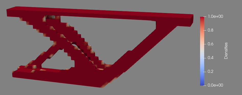
Note how even though this is a pretty simple optimization, the program still takes much longer to run in 3D than in 2D (the 3D version took about half an hour on my computer). The solution is a hollow part, and if we imagine the left half and right half of solving the same problem separately, it appears that they converged to two different solutions of the same problem. When we watch the progress of the simulation, it seems that because the right side connected from the top to the bottom in a straight diagonal line before the support beam from the bottom had the chance to connect, that support beam was extraneous and moved to the left side to complete a 3-point support. While increasing the allowed volume fraction may help, the solved solution will not be a solution to our problem which requires a volume fraction of 30%. In a broader sense, the issue we are observing is premature convergence to a local minimum. We will go in to more detail on methods of avoiding premature convergence, but for now we will fix this problem using a symmetry constraint which will make the left and right side match, since we know that the ideal geometry should be symmetric along Z as the problem definitions and bounds are symmetric as well. This limits our solution space to only symmetric solutions, and as we know the global minimum value for the objective function lies in the symmetric solution space we avoid many local minima without removing the global minimum. There are a few methods of implementing a symmetry constraint, but the simplest method is to halve the domain along Z and create a Dirichlet boundary condition along the mirror plane that prevents motion in the Z direction.

Make the following changes:

width = 25.0/2.0 # [mm]
...
    resZ = int(resolution * 2.0 * width) # Num nodes in z axis
    ...
load = Constant((0.0, -500.0/2.0, 0.0)) # [N]
...
midplane = rs.GetPlanarBoundary(\
        Point(0.0,0.0,0.0),\
        Point(0.0,thickness,0.0),\
        Point(length,thickness,0.0),\
        Point(length,0.0,0.0))
...
bc1 = DirichletBC(V, Constant((0.0,0.0,0.0)), fixedRegion)
bc2 = DirichletBC(V.sub(2), Constant(0.0), midplane)
...
u = forward_linear(rho, [bc1, bc2])

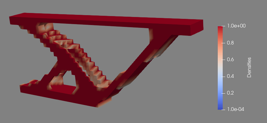
This creates a problem whose optimal solution should be able to be mirrored across the Z=0 plane to get an optimal solution to our original problem. Since the domain space is smaller now, we can also afford to increase the resolution in the Z direction to avoid problems with granularity that may arise from shrinking the domain space. After applying the threshold filter to 0.5 and a reflect filter along Z min, the generated geometry is:

Complete Code

The complete code follows and can also be downloaded here.

# Example of using Fenics to model the bending of a simple cantilevered beam in 2D.

from __future__ import print_function
import numpy as np
import region_selector_3d as rs
from dolfin import *
from dolfin_adjoint import *

E = 69000.0 # N/mm^2 - aluminum 6061
nu = 0.3 # poisson's ratio
mu = E / (2.0*(1.0 + nu))
lmbda = E*nu / ((1.0 + nu) * (1.0 - 2.0*nu))

p = 4.0 # Penalization factor
gamma = Constant(1e-2) # Min value
vf = .3 # Fraction of volume allowed to be filled

length = 250.0 # [mm]
thickness = 100.0 # [mm]
width = 25.0/2.0 # [mm]
resolution = .2 # [Nodes/mm] = 1 [Nodes/cm]
load = Constant((0.0,-500.0/2.0, 0.0)) # [N]

folder_name = './3d_cantilever_opt_results'

resX = int(resolution * length) # Num nodes in x axis
resY = int(resolution * thickness) # Num nodes in y axis
resZ = int(resolution * 2.0 * width) # Num nodes in z axis

# Boundary region for design
mesh = BoxMesh(Point(0.0,0.0,0.0), Point(length, thickness, width), resX, resY, resZ)

# Function space for displacements
V = VectorFunctionSpace(mesh, "Lagrange", 1)
# Function space for rho
V0 = FunctionSpace(mesh, "Lagrange", 1)

# Load applied on the last 4cm on the top of the beam
loadRegion = rs.GetPlanarBoundary.from_points(\
        Point(length-40.0, thickness, 0.0),\
        Point(length-40.0, thickness, width),\
        Point(length, thickness, width),\
        Point(length, thickness, 0.0))

# The end of the beam at x = 0 is fixed
fixedRegion = rs.GetPlanarBoundary.from_coord('x', 0.0)

# Mark the fixed and node loads
boundaries = MeshFunction('size_t', mesh, mesh.topology().dim() - 1)
boundaries.set_all(0)
fixedRegion.mark(boundaries, 1)
loadRegion.mark(boundaries, 2)

boundaryfile = File('%s/simpleBoundaries.pvd' % folder_name)
boundaryfile << boundaries

domains = MeshFunction('size_t', mesh, mesh.topology().dim())
# The region within 1cm of the applied load is protected, rho forced to be 1
frozenLoadRegion = rs.GetCuboidRegion(\
        Point(length, thickness, width),\
        Point(length - 40.0, thickness, width),\
        Point(length, thickness - 10.0, width),\
        Point(length, thickness, 0.0))

midplane = rs.GetPlanarBoundary(\
        Point(0.0,0.0,0.0),\
        Point(0.0,thickness,0.0),\
        Point(length,thickness,0.0),\
        Point(length,0.0,0.0))

domains.set_all(0)
frozenLoadRegion.mark(domains, 1)

domainfile = File('%s/simpleDomains.pvd' % folder_name)
domainfile << domains

ds = Measure('ds', domain=mesh, subdomain_data=boundaries)
dx = Measure('dx', domain=mesh, subdomain_data=domains) 

loadArea = assemble(Constant(1.0)*ds(2))
scaledLoad = load / loadArea

# Penalization on intermediate values
def alpha(rho):
    return gamma + (1-gamma)*rho**p

def eps(u):
    return sym(grad(u))

def sigma(u, rho):
    return alpha(rho)*(lmbda*tr(eps(u))*Identity(mesh.topology().dim()) + 2.0*mu*eps(u))

def forward_linear(rho, bcs):
    du = TrialFunction(V)
    u = Function(V, name="Displacement")
    v = TestFunction(V)

    a = inner(sigma(du, rho),eps(v))*dx(0) + inner(sigma(du, Constant(1.0)), eps(v))*dx(1)
    L = dot(scaledLoad,v)*ds(2)

    solve(a == L, u, bcs)
    return u

bc1 = DirichletBC(V, Constant((0.0,0.0,0.0)), fixedRegion)
bc2 = DirichletBC(V.sub(2), Constant(0.0), midplane)

# Initial guess: uniform density with max volume fraction
rho = interpolate(Constant(vf), V0)

# Solve initial displacement for the initial guess
u = forward_linear(rho, [bc1, bc2])

iterations = File("%s/iterations.pvd" % folder_name)

# Runs after every optimization iteration
def derivative_cb(j, dj, m):
    # Add this iteration's densities to the iterations file
    m.rename("Densities", "Densities")
    iterations << m

# Define objective functions for a minimization problem:

# Weights for each part of objective function:
dispW = Constant(1.0)
filterW = Constant(5.0e-1)

# Maximize stiffness <-> minimize displacement
Jdisp = assemble(dispW * dot(load,u)*ds(2))
# Minimize the gradient of rho <-> Reduce checkerboard problem
Jfilter = assemble(filterW * inner(grad(rho), grad(rho))*dx(0))

J = Jdisp + Jfilter

# Define control
m = Control(rho)
m_bounds = (0.0,1.0)

# Define reduced functional
Jhat = ReducedFunctional(J, m, derivative_cb_post=derivative_cb)

# Create volume constraint: Integral of rho / Area <= vf
class VolumeConstraint(InequalityConstraint):
    def __init__(self, volfrac):
        self.volfrac = volfrac
        self.smass = assemble(TestFunction(V0)*Constant(1.0)*dx)
        self.smassNotFrozen = assemble(TestFunction(V0)*Constant(1.0)*dx(0))
        self.smassFrozen = assemble(TestFunction(V0)*Constant(1.0)*dx(1))
        self.rhovec = Function(V0)
        self.rhovecFrozen = interpolate(Constant(1.0),V0)

    def function(self, m):
        from pyadjoint.reduced_functional_numpy import set_local
        set_local(self.rhovec, m) # Set rhovec to the control, rho
        integralNotFrozen = self.smassNotFrozen.inner(self.volfrac - self.rhovec.vector())
        integralFrozen = self.smassFrozen.inner(self.volfrac - self.rhovecFrozen.vector())
        
        return integralNotFrozen + integralFrozen
    
    def jacobian(self, m):
        return [-self.smass]

    def output_workspace(self):
        return [0.0]

problem = MinimizationProblem(Jhat, bounds=m_bounds, constraints = VolumeConstraint(vf))
parameters = {"max_iter": 500, 'linear_solver': 'ma97', 'tol': 1e-3, 'acceptable_tol': 1e-3, 'acceptable_iter':10}

solver = IPOPTSolver(problem, parameters = parameters)
rho_opt = solver.solve()

# Post Processing 
u = forward_linear(rho_opt, bc1)
u.rename("Displacement", "Displacement")

v2d = vertex_to_dof_map(V0)
index_inside_pad = []

# Mark all frozen regions
for i,x in enumerate(mesh.coordinates()):
    if frozenLoadRegion.inside(x,True): index_inside_pad.append(i)

rho_opt.vector()[v2d[index_inside_pad]]=Constant(1.0)
rho.assign(rho_opt)
rho.rename("Densities","Densities")

# von Mises Stress
stress = sigma(u, rho)
s = stress - (1./3)*tr(stress)*Identity(3) # deviatoric stress
von_Mises = sqrt(3./2*inner(s,s))
Vvm = FunctionSpace(mesh, 'P', 1)
von_Mises = project(von_Mises, Vvm)
von_Mises.rename("von Mises", "von Mises")

xdmf_file = XDMFFile('%s/results.xdmf' % folder_name)

xdmf_file.parameters["flush_output"] = True
xdmf_file.parameters["functions_share_mesh"] = True
xdmf_file.parameters["rewrite_function_mesh"] = False
xdmf_file.write(rho, 1.0)
xdmf_file.write(u, 1.0)
xdmf_file.write(von_Mises, 1.0)